IEEE ITSC 2026 · Accepted

Tonic Meta-Control for Adaptive Safety-Compute Allocation via Persistent Vigilance Dynamics

How a car decides when to think harder about the road ahead — and how much harder — instead of running expensive reasoning at every step.

Kyungtae Han, Yitao Chen, Nejib Ammar, Onur Altintas

Toyota Motor North America, InfoTech Labs

PDF

Autonomous Driving Compute Allocation Closed-loop Simulation

In short

A self-driving car usually needs only a cheap reflex: watch the gap to the car ahead and brake if it closes. Occasionally it needs something more expensive: check the next lane over, anticipate a cut-in, consider changing lanes. An onboard computer cannot afford the expensive option at every control step, so something has to decide when to spend it. This project is a small controller that makes that call. We tested it on scripted risk traces and in a closed-loop highway simulator, against rules that are always cheap, always expensive, or that react only to sudden surprise. It uses noticeably less compute on quiet driving; it is not uniformly safer in every scenario; and it will miss a hazard that builds up too gradually to look surprising.

Should we think harder right now?

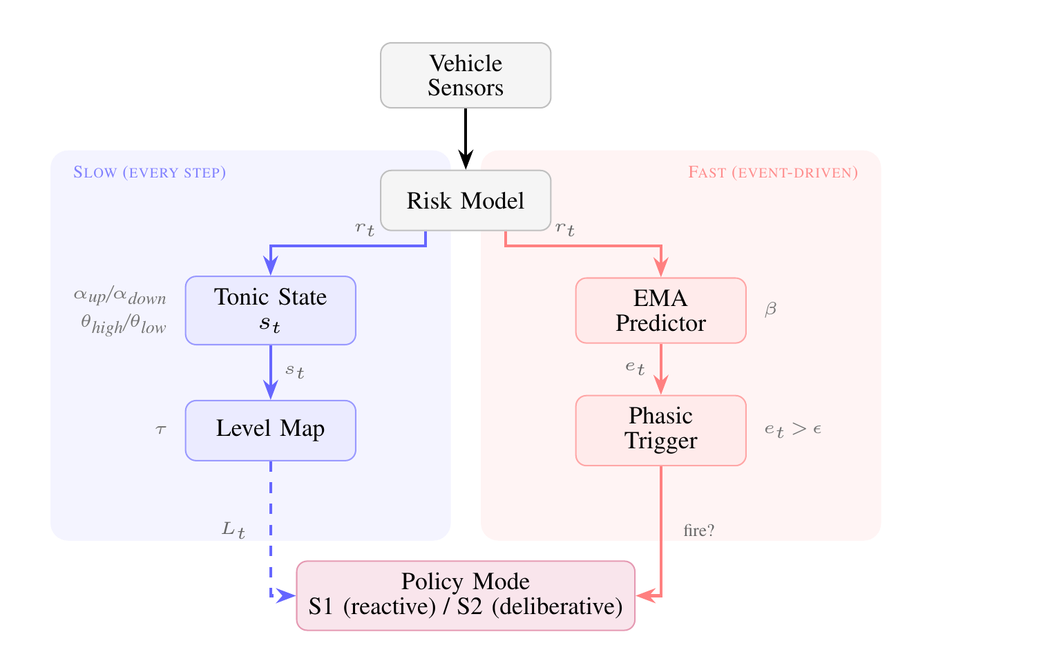
Answered by a fast check for sudden change. If the road just got worse than expected, it flips the switch on. It only decides whether to act — never how much.

How much thinking is enough?

Answered separately, by a slow running memory of how tense the last stretch of driving has been. A road that has been busy for a while earns a deeper look than one that was calm a moment ago.

Risk from the vehicle sensors feeds a slow memory path and a fast surprise path, which together select a cheap reactive mode or an expensive deliberative mode — **What you are looking at:** the risk score coming off the vehicle sensors and splitting into two paths. The left path updates a slow vigilance memory on every timestep and sets *how deep* the reasoning should go; the right path watches for a sudden jump and decides *whether* to act now. **Takeaway:** depth and timing are driven by two different signals. That separation is the whole idea. Two labels on the diagram are worth decoding: S1 and S2 are just the cheap reactive mode and the expensive deliberative mode, and the *EMA predictor* is a short running average of recent risk — the yardstick the surprise check measures against.

Update rule for the slow memory: high risk raises it, low risk lowers it, and a shaded middle band holds it exactly — **What you are looking at:** how much the slow memory moves for a given level of risk. High risk pushes it up, low risk lets it drift back down, and inside the shaded middle band it is held exactly where it is. The up arrow is steeper than the down arrow on purpose. **Takeaway:** the hold band is what stops a noisy risk score sitting near a threshold from flipping the car back and forth between modes, and the asymmetry means the system goes on alert quickly but stands down slowly.

Summary

Problem, approach, and what we ran

Problem

Always using the cheap reflex leaves the car under-prepared in dense traffic. Always using the expensive look-ahead burns onboard compute on an empty highway. Reacting only to sudden surprise forgets that a stretch of road has been busy for a while, and thrashes when a noisy risk score sits right on a threshold.

Approach

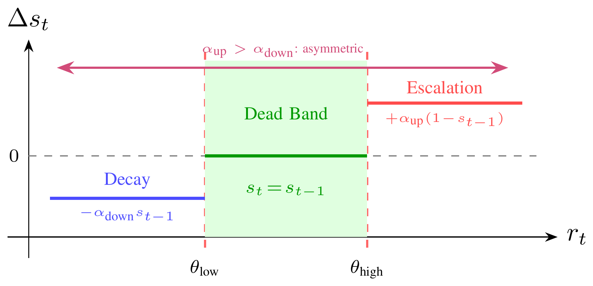
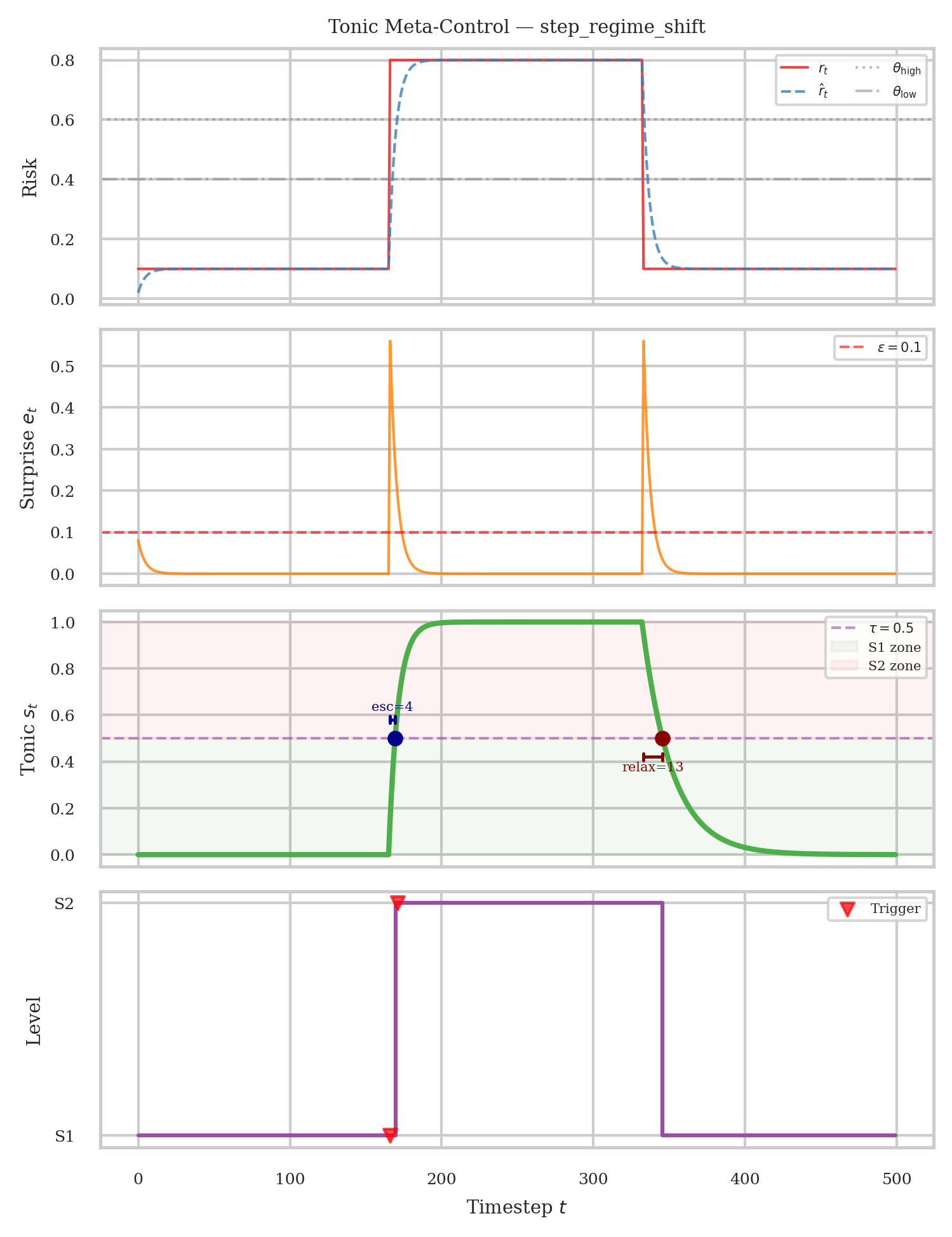
Split the decision. A slow running memory of risk — we call it the tonic state — sets how deep the reasoning goes. A separate fast surprise check — the phasic signal — decides whether to run it at all. A hold band in the middle of the risk range keeps the memory steady instead of chattering.

What we ran

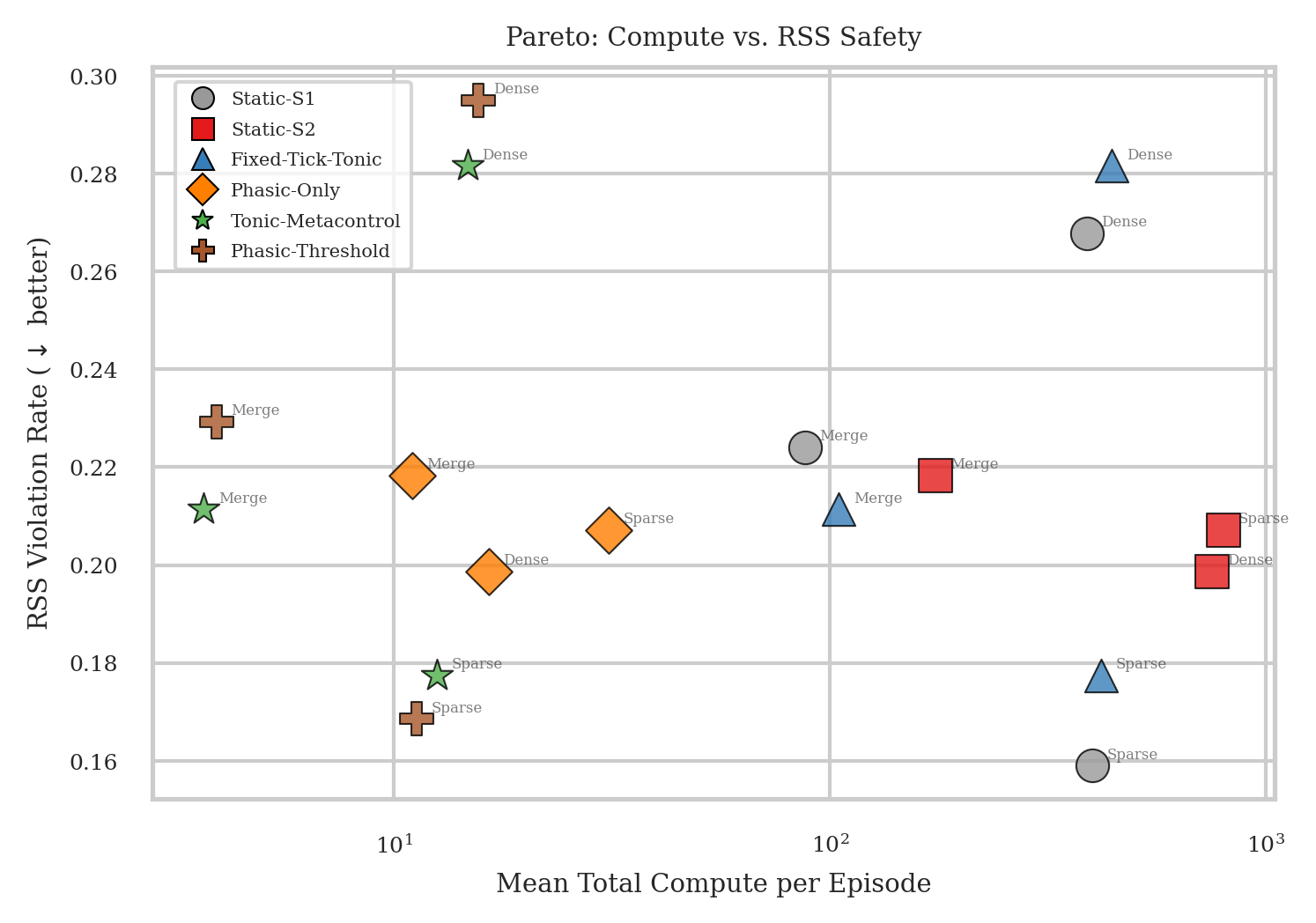
Five scripted risk patterns, then a closed-loop highway simulator in sparse traffic, dense traffic, and a merge. Six allocation rules were compared, all sharing the same perception, the same risk score, and the same underlying driving controller. The only thing that differs between them is the rule that decides how to spend compute.

Method

How It Works

On every timestep the controller does the same small amount of bookkeeping — update the memory, update the surprise estimate — and then either invokes the chosen mode or does nothing extra. The bookkeeping itself is a comparison and a multiply-add, so it is negligible next to the reasoning it is scheduling.

Keep a slow memory of how risky the road has been. Each timestep the current risk score nudges a single running value up, down, or not at all. Inside a middle band it is held exactly, so sensor noise near a threshold cannot flip the mode. It climbs faster than it decays — a deliberate bias toward staying alert, since it is cheaper to be over-prepared than under-prepared.
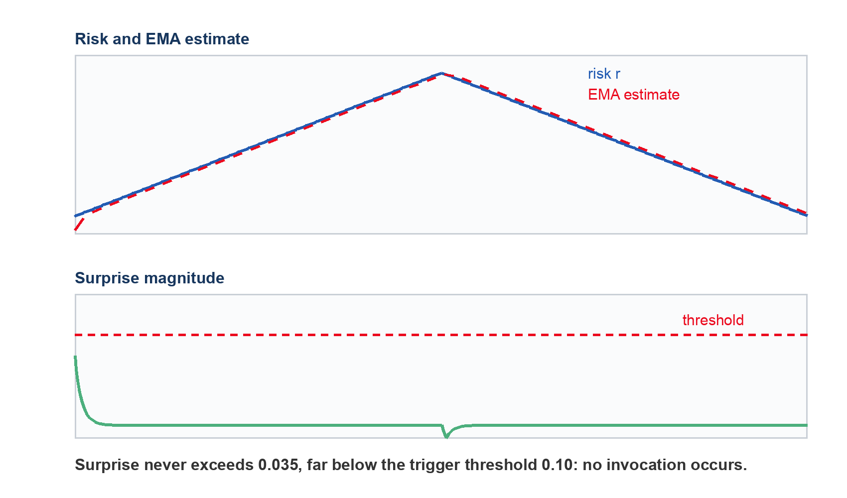
Watch separately for things getting suddenly worse. Compare the current risk against a short running average of recent risk. Fire only if the gap is large, risk is still rising, and enough time has passed since the last firing. This is purely an on/off switch — it never decides cheap versus expensive.
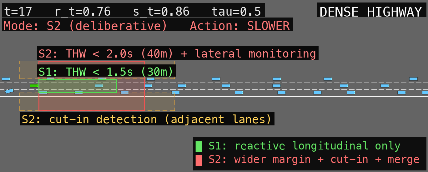
Put the two together. When the surprise check fires, the slow memory is what says which mode to run. In cheap mode the car watches the gap to the vehicle ahead and brakes. In expensive mode it looks further ahead and into the adjacent lane, so a cut-in is visible, and a lane change becomes available.

A dense highway frame with the monitored region drawn on it: the cheap mode watches only the car ahead, the expensive mode also watches the adjacent lane — **What you are looking at:** a single frame of dense highway traffic with the region the car is monitoring drawn over it. The cheap mode tracks only the gap to the vehicle directly ahead. The expensive mode looks further down the road and into the neighbouring lane, where a cut-in would come from. **Takeaway:** “spending more compute” here means literally attending to more of the road, and that is what the controller is rationing. The overlay labels S1 and S2 are the cheap and expensive modes respectively.

Experiments

What We Measured

Four stacked traces from a run where risk jumps partway through: risk and its running average, the surprise signal, the slow memory, and the resulting mode — **What you are looking at:** four stacked traces from one run in which risk jumps partway through and later falls back. Top to bottom: the risk score against its running average; the surprise signal against its firing threshold; the slow memory against the threshold that separates the two modes; and the mode the car actually ran. **Takeaway:** surprise fires only twice, right at the moments of change, while the slow memory keeps evolving in between. That is what lets depth be chosen from history rather than from whatever the sensor said this instant — and why the car escalates in a few steps but takes noticeably longer to relax.

Scatter plot of compute spent per episode against safe-distance violation rate for six methods across three scenarios — **What you are looking at:** every marker is one method in one scenario. Horizontal axis is compute spent per episode; vertical axis is how often that run violated a standard safe-following-distance rule. Further left is cheaper, lower is safer. **Takeaway:** our method lands in the low-compute region in all three scenarios, and in the merge it ties the best safety score of anything we tried. In dense traffic it stayed collision-free but did not beat the always-expensive rule on the distance metric. This is a tradeoff, not a clean sweep, and the plot is here so you can see the shape of it rather than take our word for it.

A slowly rising risk signal tracked closely by its running average, so the surprise signal never reaches its threshold — **What you are looking at:** the failure case. Risk climbs slowly and steadily instead of jumping, so the running average tracks it closely and the surprise signal stays far below its threshold. **Takeaway:** nothing ever fires, and no extra reasoning is invoked. This is not specific to our method — every surprise-triggered rule we compared does the same thing here. A periodic fallback check would be the obvious remedy; we did not build or evaluate one, so we are reporting this as an open limitation.

What this is, and what it is not

Tonic meta-control is a compute scheduler for deliberation. It sits above the driving stack and decides when the expensive reasoning path is allowed to run, and how deep it should go when it does. It is not a new object detector, not a new risk estimator, and not a new driving policy — every method in the comparison uses the same perception, the same risk score and the same underlying controller, and the only thing that changes is the rule that spends compute. The evaluation is in simulation, with a hand-built risk signal and fixed parameters; validating it against a higher-fidelity simulator and a real learned reasoning module is still ahead of us.

The paper’s own abstract, in its original technical wording.

Autonomous driving systems that incorporate deliberative reasoning modules, such as multi-step planners or large language models, face a fundamental resource allocation problem because safety demands deep inference under risk while embedded automotive platforms impose strict compute and latency budgets. We propose tonic meta-control, a mechanism that maintains a persistent vigilance state (the tonic signal, updated every timestep) via asymmetric piecewise dynamics with dead-band hysteresis. A dead-band guarantees exact state hold during boundary oscillations, providing formal guarantees on boundedness and monotonic transitions without continuous-integrator drift, and maps risk regimes to deliberation levels that govern compute allocation when rapid prediction-error surprise (the phasic signal) fires. On a synthetic testbench spanning five risk scenarios and in the highway-env driving simulator, tonic meta-control achieves 25–50% compute reduction versus phasic-only triggering, scaling to 46–52% under superlinear compute cost regimes. A memoryless threshold ablation isolates the contribution of accumulated vigilance history, confirming its advantage on transient and cyclic risk patterns. While reducing computational overhead on interactive traffic, tonic meta-control supports safety-aware autonomous reasoning on resource-constrained embedded platforms.

Cite

Citation

@inproceedings{han2026tonic,
  title     = {Tonic Meta-Control for Adaptive Safety-Compute
               Allocation via Persistent Vigilance Dynamics},
  author    = {Han, Kyungtae and Chen, Yitao and
               Ammar, Nejib and Altintas, Onur},
  booktitle = {2026 IEEE 29th International Conference on
               Intelligent Transportation Systems (ITSC)},
  year      = {2026}
}